A Masterclass in Clustering

What Is Clustering?
Clustering is a fundamental concept in machine learning, particularly in unsupervised learning. These models group similar data points together based on certain similarity measures, allowing us to gain valuable insights and patterns from unstructured data.
In this ultimate guide, I will walk you through the different types of clustering algorithms, and the key concepts behind them. We’ll also touch base upon some evaluation tactics to help understand the clusters better.
Breaking Them Down — Types of Clustering Algorithms
There are different types of clustering algorithms, each with its own bag of tricks. Let’s divide them into four categories:
Partitioning Methods
These models are like data dividers. K-Means Clustering, a supervised algorithm, is like the OG — it randomly picks a point called centroid, and groups others around them to form one non-overlapping cluster.
Then there’s Fuzzy C-Means Clustering (FCM), a bit more flexible, letting points be part of multiple clusters. Although better than K-Means clustering in handling overlapping data, it does get more computationally expensive.
In the image below, it is evident that the centroid of Cluster 2 in FCM has shifted towards the left, leading to an overlap between certain red and blue data points.

Partitioning methods are simple and efficient, but they have some drawbacks. They require us to specify the number of clusters in advance, which may not be easy or optimal. They are also sensitive to the initial choice of centroids and outliers.
Hierarchical Methods
These algorithms build a family tree of clusters. Each cluster is a node in a tree, where the root node contains all the data points and the leaf nodes contain single data points.
In Agglomerative Clustering, each data point initially exists as a standalone cluster. Subsequently, these clusters progressively merge until they ultimately coalesce into a unified entity, forming a singular cluster encompassing all data points.
On the other hand, Divisive Clustering initiates with a collective parent cluster comprising all data points. Following this, a partitioning method is employed to systematically divide this comprehensive cluster into smaller, more distinct subclusters.

Density-Based Methods
These algorithms group data points based on their density or the number of data points in their neighborhood. Data points that are in dense regions are assigned to the same cluster, while data points that are in sparse regions are considered outliers.
Density-Based Spatial Clustering of Applications with Noise (DBSCAN) looks at how crowded a spot is, and creates clusters where the party is hopping. It requires two parameters: epsilon and min_samples. Epsilon is the maximum distance between two points for them to be considered as neighbors. Min_samples is the minimum number of points required to form a dense region. It can handle clusters of arbitrary shapes and sizes, when compared to K-Means, and can detect outliers effectively. But, it may not work well for data with varying densities or high dimensions.

Ordering Points To Identify the Clustering Structure (OPTICS) is an extension of DBSCAN that does not require us to specify an epsilon parameter. Instead, it produces an ordering of the data points based on their density-reachability, which can be visualized as a reachability plot. The reachability plot shows the clusters as valleys and the outliers as peaks.

Model-Based Methods
These models assume that the data is generated by some underlying probabilistic model, such as a mixture of distributions. They try to fit the model to the data using some optimization techniques, such as maximum likelihood estimation or expectation maximization.
Gaussian Mixture Models (GMMs) assumes that the data points are generated from a mixture of several Gaussian distributions, each with its own mean and covariance. Gaussian distributions are also known as normal distributions, and they are bell-shaped curves that describe how likely a value is to occur around the mean.
The primary objective is to determine the optimal number of distributions and their parameters that best describe the dataset. This is achieved through an iterative process known as the Expectation-Maximization (EM) algorithm, where data points are probabilistically assigned to Gaussian distributions, and the parameters of these distributions are updated in turn.

How The Magic Happens — The Working Principles
These clustering algorithms group data based on similarity or distance. But how do they measure that? Let’s see.
Euclidean distance, the good ol’ formula we studied back in high school, is the straight-line route between two points in a Euclidean space. While being simple and intuitive, it may not capture the true similarity between data points if they have different scales or orientations.
Manhattan distance is like navigating the streets on a map— it is the sum of the absolute differences between the coordinates of two points in a grid-like space.

Cosine Similarity is the cosine (cos) of the angle (theta) between two vectors in a vector space. Smaller angles between two points tell us that they are very similar, while larger angles depict unrelatedness or opposite features. It is useful for comparing data points that have high-dimensional or sparse features, such as text or images.

And finally, Jaccard Similarity is the ratio of the intersection to the union of two sets. It measures the overlap of two sets, regardless of their size. It is useful for comparing data points that have binary or categorical features, such as tags or labels.

The Evaluation Party
So, you’ve thrown your clustering algorithm into the data party, but how do you know it did a good job? That’s where the metrics come in.
Internal Evaluation Metrics
Think of these metrics as the algorithm’s own self-reflection. Silhouette coefficient measures how well each data point fits into its assigned cluster, based on the average distance to other data points in the same cluster and the nearest cluster. The silhouette coefficient ranges from -1 to 1, where a higher value indicates a better fit.
The Calinski-Harabasz index and Davies-Bouldin index look at how well the clusters are behaving together. Internal evaluation metrics are useful when we do not have any prior knowledge or labels for the data.
External Evaluation Metrics
Now, imagine the algorithm getting graded by an external teacher. Purity measures how well each cluster contains only data points from a single class. Rand index measures how similar the clustering results are to the ground truth labels, while Adjusted Rand index is a normalized version of the Rand index that adjusts for chance.
Visualizing the Party
Another way to evaluate clustering quality is to visualize the clustering results using some graphical tools or techniques. Visualization can help you explore and understand your data better, as well as communicate and present your findings more effectively!
Scatter plots, heat maps, dendrograms, and techniques like PCA, t-SNE, and UMAP help you look at the clusters from different angles.

Conclusion
As you navigate the vast expanse of the data landscape, it’s crucial to recognize that clustering algorithms transcend mere tools; they stand as companions, adeptly guiding you through the intricate tapestry of patterns woven into your data. Empowered with this knowledge, your role extends beyond mere cluster analysis — you become a storyteller, unraveling the narratives concealed within each cluster.